Excel Spreadsheet Plot: Sunflower Seed Pattern Using the Golden RatioExcel Spreadsheet Plot: Fibonacci Spiral
Requirements
Reasonable knowledge of spreadsheets and an interest in the Fibonacci sequence of numbers and the Golden Ratio, Phi (φ)
Download The Excel Spreadsheet
A completed Excel spreadsheet containing the Fibonacci sequence,
sunflower seed pattern and Golden Spiral can be downloaded by clicking here. The spreadsheet is annotated to make the calculations understandable.
If you would prefer to generate your own and learn by doing, then follow the instructions below.
1. Calculate the Fibonacci Sequence of Numbers in Excel
The Fibonacci Sequence of numbers is defined as:
f(n) = f(n-1) + f(n-2)
which means that the next Fibonacci number in the sequence is the sum of the previous two. Open up a new Worksheet. Define two columns; one labelled n (index) and the other entitled Fibonacci Sequence.
The first two rows of numbers need to be entered manually to prime
the sequence, so enter the first two index numbers: 0 and 1 and the
Fibonacci numbers: 1 and 1
Your Worksheet should look like something like this: Priming the Fibonacci Sequence in ExcelClick on cell B5 and enter this formula with whatever method you prefer (typing directly or using cell selection with the mouse)
=B4+B3
Now click on cell A5 and type the number
2
Click on cell A5 and drag the mouse to B5 to highlight that data. Highlight Cells A5 & B5Drag the bottom right hand corner square down to copy the highlighted cells.
As you drag, a number in a grey square
box will be shown next to your mouse. This is the index number you have
reached during the copy operation. Drag all the way down until that
index number reaches 100.
Fibonacci Sequence Generated in an Excel Spreadsheet
And voila! You have the beginning of the
Fibonacci Sequence. Drag and copy the cells down further for more of
this infinite sequence.
2. Calculating the Golden Ratio, Phi (φ)
It can be shown that the Golden Ratio, Phi (φ) can be calculated with this formula:
The Value of the Golden Ratio
In the same worksheet that you calculated the Fibonacci Sequence, enter the Golden Ratio formula into a cell:
=(1+5^0.5)/2
The value of Phi (φ) will be calculated and displayed. You can expand the number of decimal places by right-clicking the cell > Format Cells… > Number and then increase the number of decimal places. Click OK when finished.
Alternatively, in the Home tab, look for the number group and press the button to increase decimal precision. Excel Spreadsheet: Change Decimal Precision
To 15 significant places, Phi (φ) is shown as:
1.61803398874989000
NOTE: The decimal expansion of Phi goes on forever, without a repeating pattern ever developing. This is because root 5 is used in it’s calculation and the square root of 5 is an irrational number.
However, Excel will not show decimal precision beyond 15 significant digits. Numbers are subject to truncation and are not rounded.
The highlighted red zeros are not part of the decimal expansion of
Phi. This limitation on decimal precision is a consequence of the micro
processor in your computer, which sacrifices precision for speed.
How To Increase Decimal Precision in an Excel Spreadsheet
If you want to calculate Phi to more than 15 significant places, it can be done with a spreadsheet Add-In. Visit xlPrecision to download the free edition software and read the documentation.
With the xlPrecision Add-In installed, Phi can be calculated with this formula:
=xlpDIVIDE(xlpADD(1,xlpROOT(5,2)),2)
To 100 significant places, Phi (φ) is displayed as:
3. Ratio of Adjacent Terms in the Fibonacci Sequence
The ratio of adjacent terms in the Fibonacci Sequence is an
approximation of the Golden Ratio, Phi (φ). Take a pair of adjacent
Fibonacci numbers and divide the larger number by the smaller one and
you will get a number that is very close to Phi (φ). And the further
down the Fibonacci Sequence you go, that approximation becomes
asymptotically closer to Phi (φ).
In a column next to the Fibonacci Sequence of numbers, enter Ratio of Adjacent Terms as a heading.
Click on cell C4 and enter the formula:
=B4/B3
Then copy that cell down until you reach the end of your Fibonacci Sequence on your spreadsheet. Fibonacci Sequence and Ratio of Adjacent Terms Excel Spreadsheet
It can be seen that the ratio of adjacent terms in the Fibonacci
Sequence converge on Phi (φ) very quickly. The two values are accurate
to fourteen decimal places by the 38th pair of Fibonacci numbers.
A XY scatter plot of the ratio of adjacent terms and the index demonstrate this rapid convergence. XY Scatter Plot: Ratio of Adjacent Terms of the Fibonacci Sequence
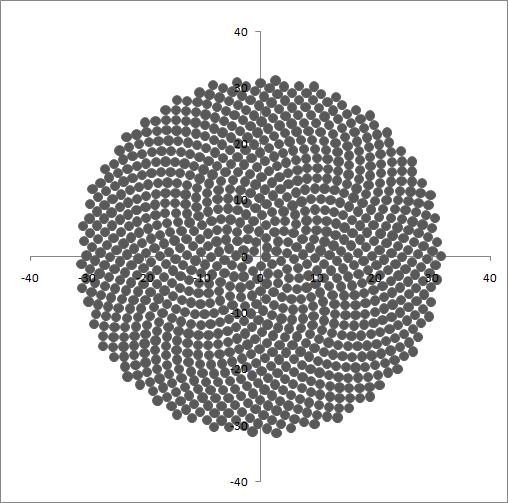
4. Plot the Sunflower Seed Pattern in Excel
Start on a fresh, blank Worksheet by clicking one of the Worksheet tabs at the bottom left of the Excel window. It’s a good idea to start renaming your tabs at this point too. Right click and select Rename to change the names of your tabs. Rename Your Worksheet Tabs
As described in Section 2, calculate the Golden Ratio (φ) with the given formula in cell B3. Calculation of the Golden Angle
The Golden Angle is the smaller of the two angles when the Golden Section is formed into a circle.
The Golden Angle: The ratio of the
whole circumference to the length of the larger arc is equal to the
ratio of the larger arc to the smaller arc.
Golden Angle
In a cell beneath your value of Phi (φ) enter this formula to calculate the Golden Angle:
=360-(360/B3)
Label your values in A3 and B3 accordingly. Values of Phi and the Golden Angle
Click on cell B4 (the value of the Golden Angle) and then write the word angle in the name box to give that value a useable name that we can reference in the next set of calculations. Naming the Value of of the Golden Angle
Now, create a series of headings as shown below: Sunflower Seed Calculation in Excel Spreadsheet
Where index starts at 1 and increments by 1.
Distance from centre is calculated by taking the square root of the index number. So the formula in cell E4 is
=SQRT(D4)
Theta is the angle at which a new seed will be generated after the
preceeding one. It is simply a multiple of the Golden Angle since it
starts at zero and increments by the value of the Golden Angle.
In cell F4, type a zero. In cell F5, enter the formula:
=F4+angle
The x,y coordinates are now easy to calculate. In cell G4, type:
=E4*COS(RADIANS(F4))
and in cell H4, type:
=E4*SIN(RADIANS(F4))
Copy all the items by dragging down to make 1,000 rows.
Create a XY scatter plot of the x and y values to generate your model of sunflower seed arrangement.
Sunflower Seed Plot in Excel
Unfortunately, Excel doesn’t realize that you’re attempting to model a
sunflower and presents you with a distorted, flattened view of your
representation. Re-size the graph and at the same time correct the
aspect ratio to make it more square.
This tutorial concludes with a method
to make Excel graphs square. A method which is required to produce an
accurate interpretation of the Fibonacci Spiral and can correct the
aspect ratio in this graph too.
Experiment with the value
of Phi (φ). Change it a little or change it a lot to see what happens to
the pattern. It becomes immediately clear that Phi (φ) is the only
number that packs the seeds into the sunflower’s head with the most
efficiency.
5. Plot the Fibonacci Golden Spiral in Excel
The Fibonacci Golden Spiral
can be approximated very closely by a logarithmic spiral that grows
away from it’s origin with a growth factor of φ with every quarter turn.
The formulae for a Golden Spiral are given as:
x = a.cosθ.ebθ
y = a.sinθ.ebθ
where a is an arbitrary scaling factor and b is the growth factor of the spiral. For the Golden Spiral:
b = ln(φ)/90 = 0.00534679805621781608330843237138
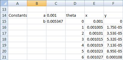
Begin in a blank Worksheet called Spiral.
Then enter the following text, values and formulae.
Golden Spiral Calculation Excel Spreadsheet
The column entitled theta simply starts at zero and increments by 1.
Taking note of my cell references, the formula for E15 is
=$C$14*COS(RADIANS(D15))*EXP($C$15*D15)
and F15:
=$C$14*SIN(RADIANS(D15))*EXP($C$15*D15)
Ensure you replicate the ABSOLUTE cell references denoted with the dollar sign ($).
Copy the theta, x and y cells down until theta reaches a value of 2173. Plot the x, y data as a XY scatter plot with lines. Excel will present something like this. A flattened Golden Spiral. The aspect ratio will be all wrong: Excel Spreadsheet: Golden Spiral Wrong Aspect Ratio
Now move on to the next step to get the aspect ratio of this graph correct.
6. How to Make Graphs Square in Excel
Excel Option ButtonClick the Excel Spreadsheet Option Button in the top left of the application window and select Excel Options.
Tick Show Developer Tab in the Ribbon if it is not ticked already. Excel Popular Options
Click OK to exit the options menu.
Click on the Developer tab in Excel. Developer Tab and ToolsClick Macros and name the macro. Any name will do. Then click Create. Create a macro
In the Visual Basic window that appears, highlight the default code and press delete on your keyboard so that nothing remains. Delete the Visual Basic CodeOpen this text file and paste the contents of it into the code window.
The macro window will look like this with the code has been copied across. Macro Code CopiedClose the Visual Basic Editor.
With the macro in place, now comes the easy bit:-
Delete the Series1 legend on your graph.
Resize your graph to occupy a large proportion of your monitor.
Ensure that your graph is selected and active.
Click Macros in the Developer tab.
Ensure that MakePlotGridSquareOfActiveChart is selected, then click Run. The aspect ratio of the selected graph will be corrected.
With the correct aspect ratio, your Golden Spiral should look something like this: Golden Spiral Plot Excel Spreadsheet Correct Aspect Ratio
Now it’s time to add the Fibonacci squares to the plot.
Click on the Insert tab and select Shapes. Choose a rectangle. Select a Rectangle from the Shapes Button
Using care, draw in the Golden Rectangle so it fits the Spiral, snugly. Draw the Golden Rectangle to Fit the Extremities of the SpiralRight click the rectangle and select Format Shape… to increase Transparency with the slider so that the Spiral can be seen.
When you are happy with the fit, choose another rectangle, hold down the shift key and draw in the first square. Take care to ensure all your lines are aligned. Use the View tab and Zoom feature for more accuracy if you need it. Alter the color and transparency of your new square. First Fibonacci Square Drawn on the Golden Spiral Plot
Continue to draw in the smaller squares. Remember to hold down the shift key before you start drawing any of the squares. This will prevent you from drawing rectangles.
Ultimately, your Golden Spiral, Golden Rectangle and Fibonacci Squares will look something like this when you are done. Excel Spreadsheet Plot: Fibonacci Spiral
If you’ve enjoyed this tutorial, please take a look at another article of mine based upon the misconceptions and use of the Golden Ratio in photography. I’m collecting data there to determine if the Golden Rectangle is indeed, the one most desired over any other rectangle.


1 Comments
Excellent post. THANK YOU... so surprised that no comments here...
ReplyDeleteGood day precious one, We love you more than anything.